To measure is to know (if you know what you are measuring).

To determine a sound level properly, it is essential to understand what kind of noise you are dealing with, how and where it is measured, and which other sources may influence it. Without this context, measurements can easily lead to the wrong conclusions.

Different countries and sectors apply their own standards to prescribe measurement methods. This article highlights the most important recurring aspects and explains how each of them can influence the outcome of a measurement.

One important element is measurement notation, which we explained in detail in our previous blog. If you are not yet familiar with terms like dB(A), LCmax, or LAeq, we recommend starting there for a quick refresher before diving deeper into this article.

Type of sound and time weighting

Time weighting and averaging methods are used to make fluctuating noise levels easier to interpret and compare. The most common are Fast (F), Slow (S), and the energy-based average Leq. Their main difference lies in the period over which averaging takes place and in how the averaging is calculated.

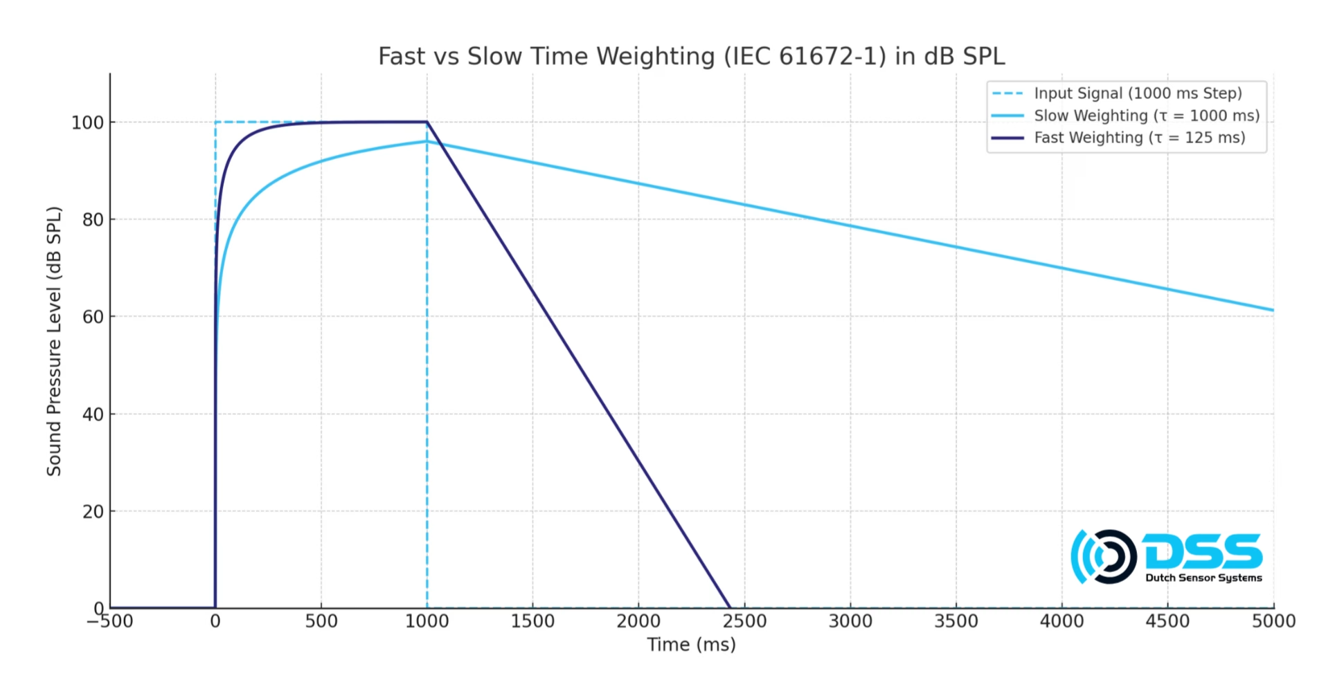
• Fast weighting applies an exponential time average with a time constant of 125 ms (⅛ of a second). This makes it sensitive to rapid changes in sound level, ideal for capturing short pulses or bursts such as impact tools in a workshop or containers clunking during loading.
  
  However, for continuous or background noise, Fast can be less useful as the displayed values fluctuate quickly above and below the average. Fast is often combined with a maximum-hold function, which records the highest level over a measurement period. This provides insight into the loudest moments that may be missed in real time. Maximum values are usually noted as LAFmax, LCFmax, etc.
  
• Slow weighting uses an exponential average with a 1-second time constant. It smooths out short-term fluctuations and gives a steadier reading. While it does not accurately represent individual short pulses, it is well-suited to relatively constant noise sources such as fans, motors, or road traffic.
  
  
• Leq (Equivalent Continuous Sound Level) is a time-integrated average of the total sound energy over a chosen period, such as 1 minute (LAeq,1min). Measurement periods are often configurable, ranging from minutes to days (or even longer, depending on the instrument).
  
  Leq condenses fluctuating noise into a single continuous level with the same total energy as the varying sound. It is particularly useful for assessing overall exposure, for example measuring the average noise level of a complete work shift.
  
  One limitation is that short but very loud events are “spread out” across the whole period, so they may not be visible in the result. For this reason, Leq measurements are often accompanied by Lmax values, especially when peak events are relevant for health or nuisance assessments.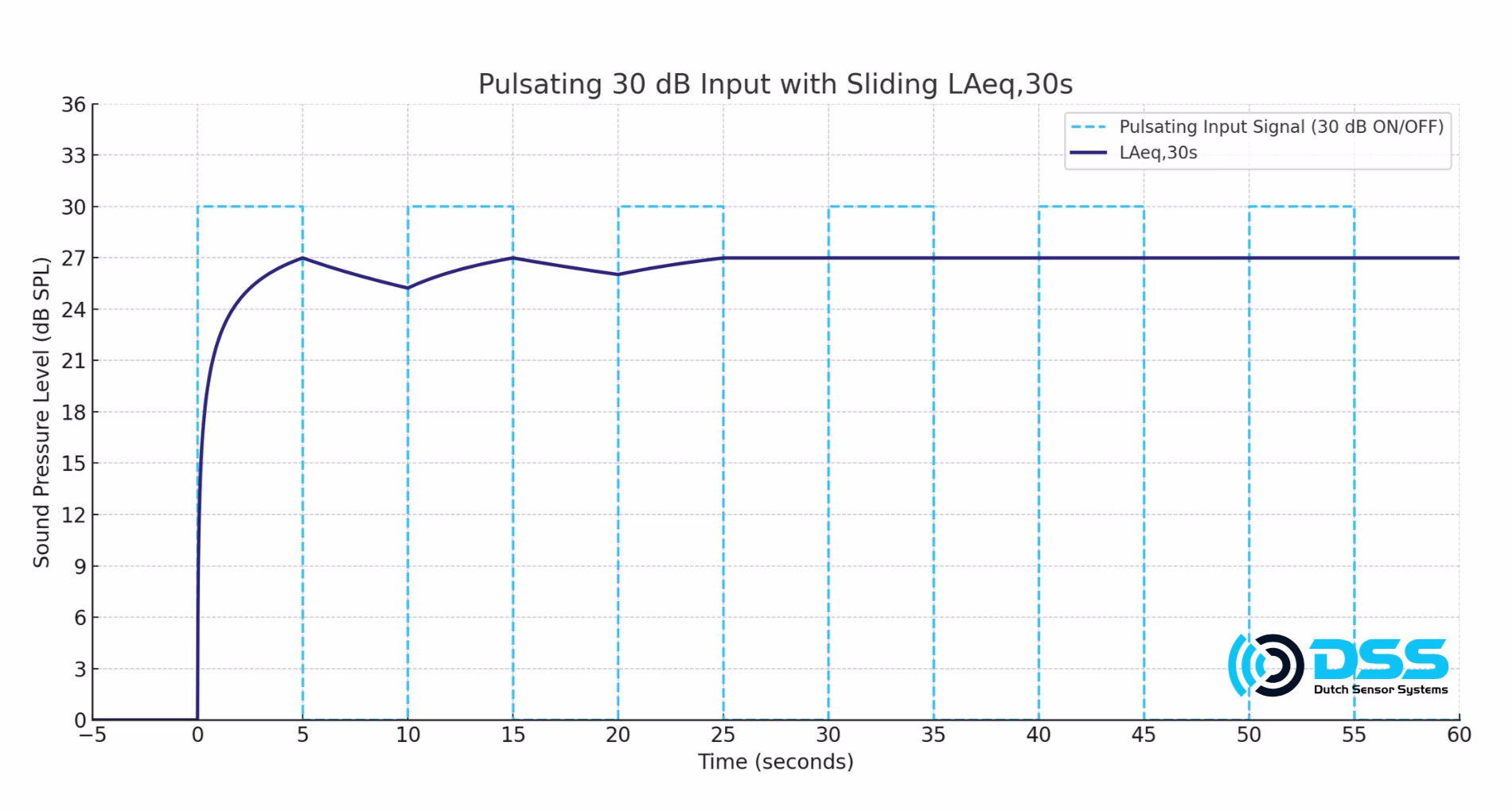
  
  

A mismatch between the type of sound and the chosen time weighting can lead to misleading results. If short, loud impulses are measured with a slow or Leq weighting, their impact may be averaged out and underestimated. Conversely, using a fast weighting on steady background noise can make the measurement appear unstable and unrepresentative. Choosing the wrong combination therefore risks overlooking critical noise events or mischaracterizing continuous exposure, reducing the reliability of the assessment.

Type of sound and frequency weighting

Frequency weighting adjusts sound measurements to better match how human hearing perceives different frequencies. These weightings are derived from the equal-loudness contours defined in ISO 226, which describe how sensitive we are to different frequencies at various loudness levels. All weightings are aligned at 1 kHz, which also serves as the standard reference for sound level calibration.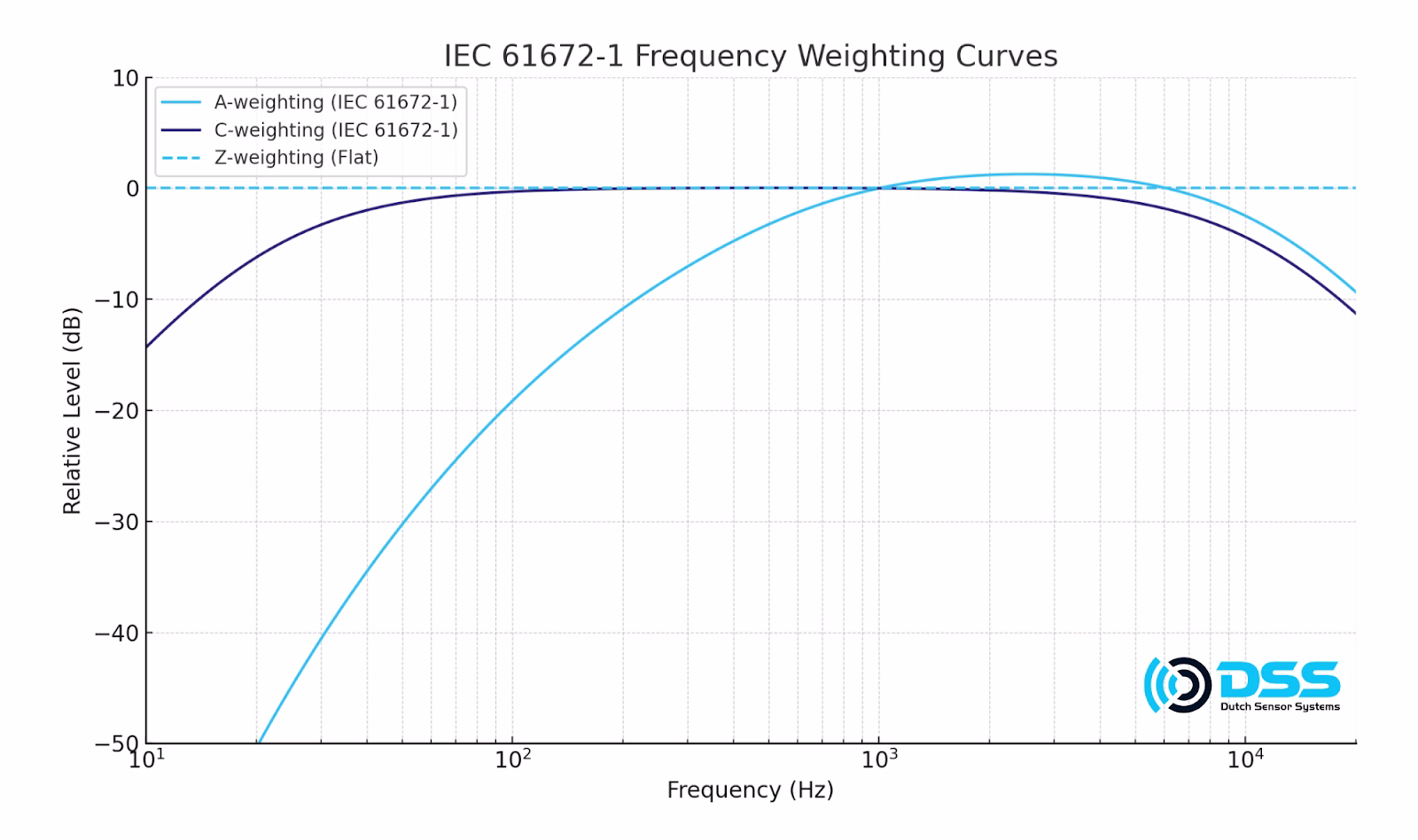

• A-weighting is based on the 40-phon contour. It is used in most everyday and regulatory noise measurements because it represents how we perceive sound at moderate loudness levels. Its key feature is the strong attenuation of low frequencies, which makes it less suitable when low-frequency noise is important. For example, the hum of an electric motor at 50 or 60 Hz will appear at least 25 dB lower in an A-weighted measurement compared to a C-weighted one.
  
• C-weighting is based on the 100-phon contour. It is applied when sound levels are very high or when low-frequency energy plays a significant role. With its flatter frequency response, it captures bass and powerful sounds more accurately. Common applications include industrial noise monitoring and concert sound measurement.
  
• Z-weighting stands for “zero” or flat weighting, meaning no frequency adjustment is applied. It is often used in technical analysis, infrasound measurements, instrument calibration, or whenever the full, unaltered frequency content of the sound is required.
  

The difference between results obtained with different frequency weightings can provide insights into the spectral balance of the noise. For instance, if a C-weighted value is significantly higher than the A-weighted one, this indicates a strong low-frequency component. Similarly, comparing C and Z can highlight the presence of very low or very high frequency noise that A and C might underrepresent.

We conducted a simple test with different types of sounds. The results clearly show how time and frequency weightings can lead to very different outcomes, even when measuring the same source:

• Red, background noise: a relatively steady sound with some low frequency content. Little difference between time weightings, some difference between A and C. 
• Green, music: very dynamic and a lot of low frequency content. Large differences between average and max, large differences between A and C.
• Blue, 1kHz tone: Steady, single frequency tone. This is where the A and C filters have equal sensitivity, there is no difference between any weighting.
• Yellow, 125Hz tone: Steady, single frequency tone. Here C is more sensitive than A, there is a lot of difference between frequency weightings, but little difference between time weightings.

Closing reflection

Understanding how time and frequency weighting shape results is only the beginning. These fundamentals lay the groundwork for reliable sound monitoring, whether in industrial compliance, workplace safety, or urban planning. In the next part of this series, we will take the discussion a step further and explore additional aspects that determine how meaningful and actionable your noise data truly is.